On Network Design Spaces for Visual Recognition
In this paper, author introduce new comparison paradigm of distribution estimates. Compared to comparing point and curve estimates of model familes, distribution estimates paint a more complete picture of entire design landscape
Introduction
There has been a general trend toward better empiricism in the literature on network architecture.
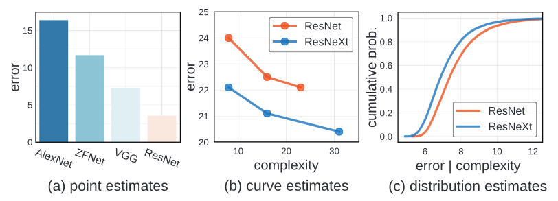
In the early development stages, the simple method was used. The progress of the neural network was measured by simple point estimates. The architecture was marked superiror if it achieved lower error on a benchmark dataset, often irrespective of model complexity.
The improved methodoloy adopted in more recent work compares curve estimates. This methods explore design tradeoffs of network architectures by instantiating a handful of models from a loosely defined model familes and tracing curve of error vs. model complexity. In this estimation, one model family is considered superior if it acheives lower error at every point along a curve. In this example, ResNeXt are considered better than ResNet because, ResNeXt have lower error in all the point.
However, there is some draw back in using this methodology. Curve estimates does not consider confounding factors, which may vary between model familes and may be suboptimal for one of them.
Rather than varying a single network hyperparameter while keeping all others fixed, what if instead we vary all relevant network hyperparameters? However, this is not feasible, because there are often infinite number of possible models. Therefore, author introduce a new comparison paradigm: that of distribution estimates.
Unlike Curve estimates where they compare a few selected members of a model family, distribution estimates sample models from a design space, parameterizing possible architectures, giving rise to distributions of error rates and model complexities.
This methodology focuses on characterizing the model family. Thus enable research into designing the design space for model search.
Related Work
Reproducible research
There has been an encouraging recent trend toward better reproducibility in machine learning. Thus author share the goal of introducing a more robust methodology for evaluating model architectures in the domain of visual recognition
Empirical studies
In the absence of rigorous theoretical understanding of deep networks, it is imperative to perform large-scale studies of deep networks to aid development. Empricial studies and robust methodology play crucial role in enabling progress toward discovering better architectures.
Hyperparameter search
General hyperparameter search techniques address the laborious model tuning process in machine learning. In this work, author propose to directly compare full model distributions not just their minima.
Neural architecture Search
NAS has proven effective for learning networks architectures. A NAS instantiation has two components: a network design space and a search algorithm. Most work on NAS focuses on the search algorithm. However, in this work, author focus on characterizing the model design space.
Complexity measures
In this work, author focus on analyzing network design space while controlling for confounding factors like network complexity. Author adopt commonly-used network complexity measures, including number of model parameters or multiply-add operations.
Design Spaces
Definitions
Model family
A model family is large (possibly infinite) collection of related neural network architectures, typically shraing some high-level architectural structures or design principles (residual connections)
Design Space
Performing empirical studies on model families are difficult since they are broadly defined and typically not fully specified. To make disctinction between abstract model families, design space is introduces. Design space is a concrete set of architectures that can be instantiated from the model family.
A design space consist of two components
- parameterization of a model family
- a set of allowable values for each hyper parameters.
Model distribution
As design space can contain an exponential number of candidate models, exhaustive evaluation is not feasible. Therefore, from a design space, author sampled and evaluated a fixed set of models, giving rise to a model distribution. Then, author use classical statistics for analysis. Any standard distribution, as well as learned distributions like in NAS, can be integrated into our paradigm.
Data Generation
To analyze network design spaces, author sample and evaluate numerous models from each design space. In doing so, author generate datasets of trained models upon which we perform empirical studies.
Instantiations
Model family
Author study three standarad model families:
- Vanilla model family (feedforward network loosely inspired by VGG)
- ResNet model family
- ResNeXt model family
Design space
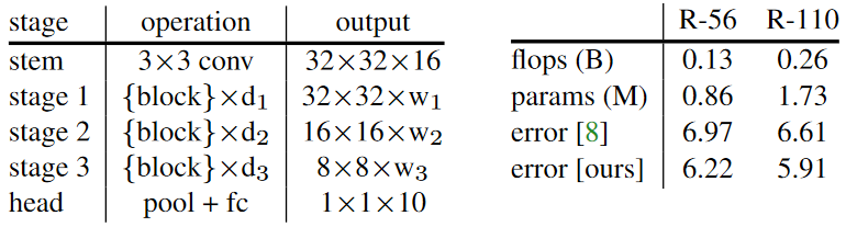
As shown in the table above, author used networks consisting of a stem, followed by three stages and a head, as described in the table above.
- For ResNet design space, a single block consists of two convolutions and residual connection.
- Vanilla design space uses an identical block structure as ResNet but without residual connection.
- In the Case of ResNeXt design spaces, we use bottleneck blocks with groups.
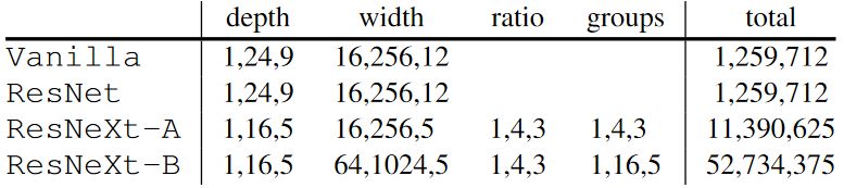
This table above specify the set of allowable hyperparameters for each. The notation, means we sample, n values sapced about evenly in log spaces in the range a to b. From these value, we select independently for three network stages, number of blocks
, and the number of channels per block
.
From these number, the total number of models is for models without groups and
for models with groups.
Model distribution
Author generate model distributions by uniformly sampling hyperparameters from the allowable values for each design spaces.
Data generation
Author uses image classification models trained on CIFAR-10. This setting enables large-scale analysis and is used often used as a testbed for recognition networks. From the above table, author selected 25k models and used to evaluate the methodology
Proposed Methodology
Comparing Distribution
When developing a new network architecture, human experts employ a combination of grid and manual search from a design space, and select the model achieving the lowest error. The final model is a point estimate of the design space.
Comparing design spaces via point estimates can be misleading. This is illustrated by comparing two sets of models of different sizes sampled from the same design space.
Point estimates
The baseline model set (B) by uniform sampling 100 architecure from ResNet design space described above. The second model set(M) uses 1000 samples instead of 100. The difference in number of samples could arise from more effort in the development of M over the baseline, or simply access to more computational resources for generating M. These imbalanced comparisons are common in the practice.
After traing, M’s minimum error is lower than B’s minimum error. Since the best error is lower, a naive comparison of point estimates concludes that M is superior.
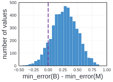
Repeating this experiment yield the same results. Above image represent the difference in the minimum error of B and M over multiple trials. This experiment was simulated by repeatedly sampling B and M from the pool of 25k pre-trained models.
In 90% of the cases M has a lower minimum than B, often with large margin. However, M and B were drawn from the same design space. Thus using point estimation can be misleading.
Distributions
Author argues that one can estimate more robust conclusion by directly comapraing distributions rather than point estimates such as minimum error.
To compare distributions, author use empirical distribution functions(EDFs). Given the set of n models, with errors , the error EDF is given as following:
This equation represent the fraction of models with error less than e.
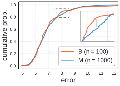
Using B and M, author plotted the empirical distribution instead of just their minimum errors. The small tail to the bottom left indicate a small population of models with low error and the long tail on the upper right shows there are few models with error over 10%.
Quanlitatively there is little visible difference between the error EDFs for B and M, suggesting that these two set of models were drawn from an identical design space.
To make quantitative comparison, use Kolmogorove-Smirnov test, a nonparametric statistical test for the null hypothesis that two samples were drawn from the same distributions. Given and
, the KS statistic D is defined as:
D measures the maximum vertical discrepancy between EDFs(the zoomed panel in the graph); small value suggest that and
are sampled from same distribution. In this experiement, the KS test gives
and a p-value of 0,60. Thus from this result we could assume that B and M follow the same distribution.
Discussion
The above example demonstate the necessity of comparing distributions rather than point estimates, as the latter can give misleading results in even simple cases.
The most work reports results for only a small number of best models, and rarely reports the number of total points explored during model development, which can vary substantially.
Controlling for Complexity
While comparing distributions can lead to more robust conclusions about design spaces, comparison must done between controlled confounding factors that correlate with model error to avoid biased conclusions.
Relevant confounding factor is model complexity. The next section study how to control the complexity of the model.
Unnormalized comparison
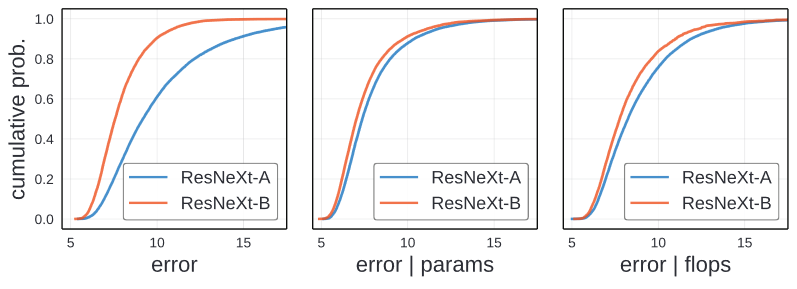
The leftmost image shows the error EDFs for the ResNeXt-A and ResNeXt-B design spaces, which only differes in the allowable hyperparameter set in the above table.
Looking through the image, qualitative difference is visible and suggest that ResNeXt-B is a better design space. For every error, EDF for ResNeXt-B is higher at every error threshold.
This image present that different design space from the same model family under the same model distribution can result in very different error distributions.
Error vs Complexity
Though different papers, we know that model’s error is related to it’s complexity; in particular more complex models are often more accurate.
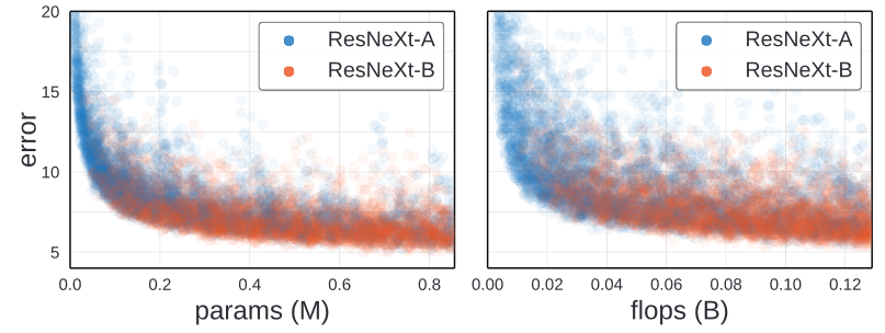
This two graphs plot the error of each trained model against its complexity, measured by either parameter or flop count. While there are poorly-performing high-complexity models, the best models have the highest complexity.
Complexity distribution
The difference between the ResNeXt-A and ResNeXt-B might be due to the differences in their complexity distributions.
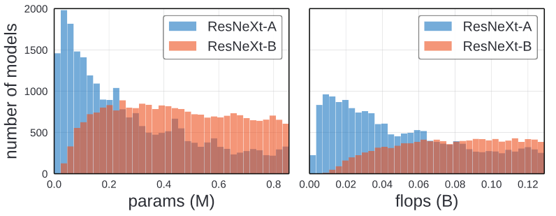
As shown in the image above, ResNeXt-A have more low compelxity models and ResNeXt-B have heavy tail of high-complexity models. Thus, it is plausible that ResNeXt-B’s apparent superiority is due to the confounding effect of complexity.
Normalized Comparison
Author propose a normalziation procedure to factor out the confounding effect of the differences in the complexity of model distributions.
Given a set of n models where each model has complexity , the idea is to assign to each model a weight
, where
to create a more representative set under that complexity measure.
From using above parameters, we define normalized complexity EDF as
Likewise the normalized error EDF is defined as :
From given two model set, our goal is to find weights for each model set such that for all c in a given complexity range. After finding the weights, comparison between
and
reveal the difference between design spaces that cannot be explained by model complexity alone.
In the Figure found on section Unnormalized comparison, the middle and right image is normalized by parameters and flops. Controlling the complexity brings the curve closer. However, the small gap between ResNeXt-A and ResNeXt-B might caused by higher number of groups and wider width.
Characterizing Distributions
An advantage of examining the full errror distribution of a design space is it gives insights beyond the minimum achievable error. Examining distributions allows us to more fully characterize a design space.
Distribution shape
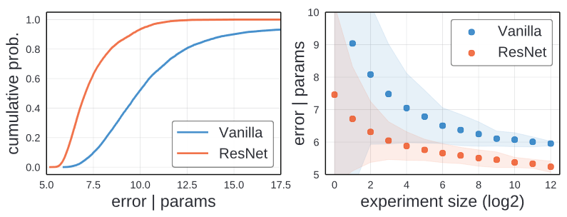
The left image shows EDFs for the Vanilla and ResNet design space. For ResNet majority(>80%) of the model have error under 8%. In constrast, the Vanilla design space has a much smaller fraction of such models(~15%). This represent it is easier to find a good ResNet model.
Distribution area
EDF can be summarized by the average area under the curve up to max . By this we could compute :
However, the area gives only a partial view of the EDF.
Random Search Efficiency
Another way to assess the ease of finding a good model is to measure random search efficiency.
To simulate random search experiments of varying m, author sampled m models from our pool on n models and take their minimum error. Then repeat the process n/m times to obtain the mean along with the error vars for each m. To eliminate confounding effect of complexity, weight is assigned to each model.
In the right of the above graph, random search was used on both Vanilla and ResNet to simulate random search. Using random search finds better models faster in the ResNet design space.
Minimal Sample Size
In practice far fewer samples can be used to compare distrubtions of models as we now demonstrate.
Qualitative analysis
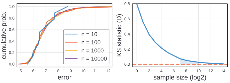
Left image shows EDFs for the ResNet design space with varying number of samples. Using 10 samples to generate EDF is quite nosizy, However, 100 samples gives reasonalbe approximation. 1000 sample is indistinguishable from 10000. Thus author suggest to use 100 to 1000 samples.
Quantitative analysis
For quantitative analysis, we compute the KS statistic D between full smaple of 25k models and sub samples of increasing size n. The right image above is the result of the comparison. At 100 samples D is about 0.1 and at 1000, D begins to satuate. Beyong 1000 samples, shows diminishing returns.
Thus as qualitative analysis, using sample size between 100 and 1000 is a reasonable sample size.
Feasibility discussion
Some might wonder about feasibility of training between 100 and 1000 models for evaluating distribution. In authors setting, Training 500 CIFAR models required about 250 GPU hours. In comparison, Training a typical ResNet-50 baseline on ImageNet requires about 192 GPU hours.
Therefore, evaluating the full distribution for a small-sized problem like CIFAR requires a computational budget on par with a point estimate for a medium-sized problem like ImageNet
Overall, distribution comparison is quite feasible under typical setting.
Case Study: NAS
As a case study of distribution estimation, author examime design space from recent neural architecture search(NAS) literature.
NAS has two core components:
- a design space
- a search algorithm over design space
Design Spaces
Model family
NAS model is contructed by repeatedly stacking a single computational unit. A cell can vary in the operations it performs and in its connectivity parttern.
A cell takes output from two previous cells as inputs and contains a number of nodes. Each nodes in a cell takes as input two previously constructed nodes, applies an operator to each input, and combines the output of two operators.
Design Space
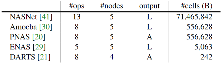
From five different NAS model family, NASNet, AmoebaNet, PNAS, Enas, and DARTS was selected. As shown in the table above, most of the NASNet is limited to have five cell structure. The Output L means, loose node not used as input to other nodes, and A all nodes are concatenated to the output.
The full network architecture also varies slightly between recent papers. Thus author standardized this aspect of design spaces. The network arhitecture setting from DARTS was adopted.
The network depth d and initial filter width are typically kept fixed. However these hyperparameters directly affect model complexity.
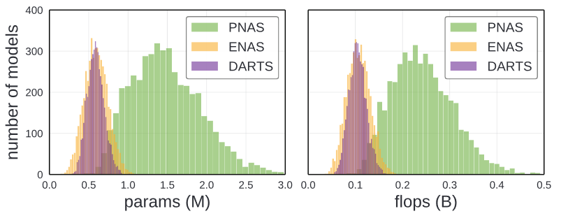
As Shown in the image above, each model generates different complexity. Therefore to factor this confounding factor, author vary w and d ( and
).
Model Distribution
Author sampled NAS cells by using uniform sampling at each step. Likewise w and d is uniformly sampled.
Data Generation
Training approximately 1000 CIFAR models for each of the Five NAS design spaces. Ensure 1000 models per design space for both full flop range and full parameter range.
Design Space Comparison
Distribution comparison
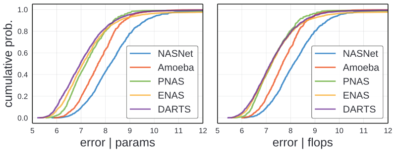
Above image show normalized error EDFs for each of the NAS design spaces. The NASNet and Amoeba design space are noticeably worse than the others, while DARTS is best overall. Comparing ENAS and PNAS, they are similar but ENAS has more intermediate error while Enase has more lower/higher performing models.
Author thinks the gains in each paper may come from improvements of the design space.
Random Search efficiency
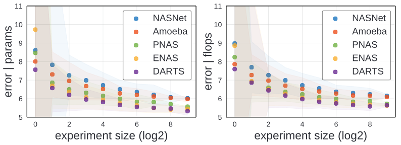
From above image, we observe two interesting facts.
- The ordering of design spaces by random search efficiency is consistent with the ordering of the EDFs.
- For a fixed search algorithm, the differences in the design space leads to clear difference in performance.
Comparisons to Standard Design Spaces
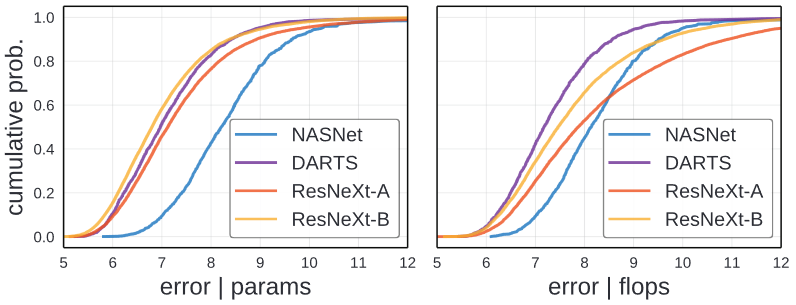
From selecting best and worst performing NAS design spaces(DARTS and NASNet) and compare them to the ResNeXt design spaces. ResNet-B is on par with DARTS when normalized by parameter( as shown in the left), while DARTS slightly outperforms ResNeXt-B when normalized by flops(as shown in the right).
These result demonstarate that the design of the design space plays a key role and suggest that designing design spaces, manually or via data-driven approaches is a promising avenue for future work.
Sanity Check: point Comparison
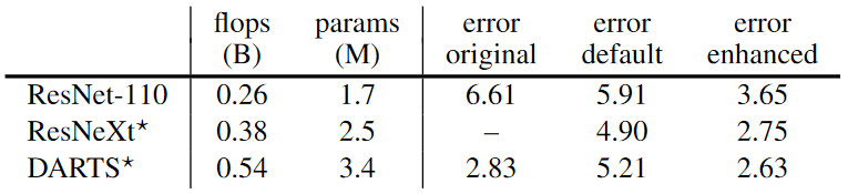
As a sanity check, author perform point comparisons using larger models and the exact training setting from DARTS with deep supervision, Cutout and modified DropPath. DARTS, ResNeXt, and ResNet-110.
The result presented in the above table. With enhanced setup, ResNeXt achieves similar error as DARTS.
Conclusion
Author present methodology for analyzing and comparing model design space. This methodology should be applicable to other model types, domains, and tasks.